Whatcha reading today, doc?!

Welcome to BookLook! BookLook is a recommender system for book readers which aims to assist users in the task of finding the next book to read. BookLook will take into account both the dislikes and likes of the reader and his/her friends to recommend the “Next book to read”.

Dataset

The dataset used is Book-Crossing dataset available in [2]. The Book-Crossing dataset contains 278,858 users (anonymized but with demographic information) providing 1,149,780 ratings (explicit / implicit) about 271,379 books. This dataset was collected by Cai-Nicolas Ziegler in a 4-week crawl from the Book Crossing community. The Book-Crossing dataset comprises of 3 tables: BX-Users, BX-Books, BX-Book-Ratings. We used the BX-Book-Ratings table for our implementation. We use 50,000 users x 50,000 books and create a bipartite graph using NetworkX.

Methodology

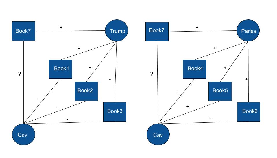
To take advantage of the dislikes of the user, we plan to use the method of 'Love-Hate Square Counting Method' proposed in [1] Let's take an example to explain this! Suppose Cav is friends with Trump and Parisa. Now, Cav hates 3 books which Trump also hates & Cav loves 3 books which Parisa also loves. Now if we know that Trump likes "Twilight" and Parisa likes "Life of Pie", then , is it more likely for Cav to like "Twilight" or "Life of Pie"? This is exactly the question we are trying to answer with BookLook!

Related Work

There are existing book recommending systems in the market. Goodreads is one such example, it provides personalised recommendations based on user interests and collaborative models. These recommendations are based on books the user recently shelved, and from the overall ratings of books provided by all the users on the platform. However, Goodreads does not seem to take into account the likes and dislikes of a user’s friends while recommending books to the user. BookLook does take this dislike/hate feature into account. [1] talks about how the most powerful signal in predicting a user’s high rating of an item comes from what items he or his friends dislike.

Love-Hate Square Counting Method

The Love-Hate Square Counting method is implemented with a bipartite graph. This method is more like a network-based Collaborative filtering. We represent the users as one set of nodes and the items (books) as another set of nodes and form the bipartite graph. The edges between the user and the item are classified as Love (+) if the user's rating for the item is more than 7 and Hate (-) if the rating is less than or equal to 7.

We perform BFS on this graph to get configurations. Assume we have a target user ut and a target item ti. The recommender system is now expected to predict the preference of the user ut with respect to the item ti depending on the information available. The Love-Hate Square Counting Method does this by taking into account the neighboring users of the uset ut. A user must satisfy the following conditions to be a neighbor of the target user ut.

1) The user must have rated the target item ti.
2) The user must have rated an item or items which the targer user ut has also rated.

Now the frequency of all the possible configurations are found by performing a BFS traversal on the bipartite graph. Assuming the intermediate user to be ot and intermediate item to be oi, the possible configurations are as shown below.

The frequency of all the possible configurations are counted and the represented as a feature vector with 8 features. This feature vector is then fed into a Machine Learning model to train and the model is tested for accuracy.

Evaluation

We use Naive Bayes, Logistic Regression, SVM, Decision Trees and KNN to classify and predict whether the target user loves or hates the target item. We see that SVM and Logistic Regression perform the best of all. We used the classic method of prediction, the Matrix Factorization method to evaluate our love-hate model. The SVD model was implemented and it was found that the RMSE values are actually lesser for the LHSCM and the recall values for hate were not that great for SVD. Hence, our model performs better than SVD giving a RMSE of 0.62 for Logistic Regression and a recall value of 0.95 for hate for SVM. A point here to be noted is that we want the recall value for hate to be high, so that nothing which is actually hated is seen as love and recommended to the user!

Neural Networks: RBM

We go beyond our model to construct a neural network using Restricted Boltzman Machines (RBM) which constructs the feature vectors by itself when trained. An RBM network is an undirected bipartite network with visible nodes on one side and hidden nodes on the other side with the edges between them as weights. Think of the visible nodes as Books and the hidden nodes as latent factors (eg: genre, author, bestseller etc.). The network goes on in training by updating the weights from visible to hidden nodes in one iteration and then updating the weights again from hidden to visible nodes in the next iteration and so on. During testing, we evaluate the model on the latent vectors/feature vectors that the network learnt by itself during training. We see that RBM improves the RMSE to 0.58, which is the least for all the models tested by us.

Code Logistics

The ipynb files with the code can be found in the below location. There are 3 separate files in the location. The file BookLook_final.ipynb is the file that has the LHSCM implememntation. The BookLook_SVD.ipynb is the file that has the SVD model implementation and BookLook_RBM has the Neural network model implementation.
https://github.com/fnumegha/BookLook/tree/master/Code

BookLook A recommender system for books